| |
| open all |
| fold all |
| line height: |
| font size: |
| line width: |
| (un)justify |
| replicate |
| highlite |
| refs |
| contents |
| purge |
Contents
1. Preface

Configurations of Skew Lines
Julia Viro and Oleg Viro
Key words and phrases. Projective configurations, skew lines, isotopies and rigid isotopies, mirror configurations, join
Mathematics Subject Classification. Primary 51H10, 51A20; Secondary 05B30, 51E30
Abstract
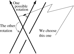
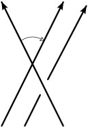
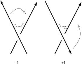
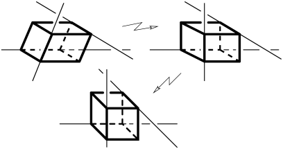
The expanded version [Viro and Drobotukhina 1989] of [Viro and Drobotukhina 1988] was published in the first volume of a Russian journal Algebra i Analiz opening a new section “Light reading for the professional”. English version of the paper became available in a translation made by N. Koblitz and published by American Mathematical Society in the first volume of Leningrad Mathematical Journal. Unfortunately, the first volumes, even of the first rate journals, are not distributed as well as they deserve. Leningrad Mathematical Journal is an excellent journal, but we would like to bring our paper to more readers. During 16 years which passed since the time of writing [Viro and Drobotukhina 1989] some questioned posed in [Viro and Drobotukhina 1989] were solved and we decided to refresh the text and make it available to new readers. Partly we fix here some of defects of [Viro and Drobotukhina 1989] : wrong pictures and few terminological inaccuracies of translation. Furthermore, some of the results appeared in other papers without appropriate references. The tradition of wrong priority references was established in papers by R. Penne and H. Crapo [Penne 1993] , [Crapo and Penne 1994] . We expanded the bibliography for the sake of completeness, but arranged it in the chronological order, to facilitate orientation in the history of the subject. Any set of disjoint line segments can be moved around to any other relative location in such a way that they remain disjoint. This we can see from experience, and it is also not hard to prove. We depict straight lines using line segments, and so it seems to us that straight lines cannot be woven together. But is that really the case? First of all, let us give a more precise statement of the questions which concern us. The first question is: Can a set of disjoint lines be rearranged? But what do we mean by the term “rearrange”? Here we shall not be concerned with the angles or distances between the lines. We shall consider the relative position of the lines to be unchanged if we move them in such a way that they never touch. But if one set of lines cannot be obtained from another set by such a movement, then we shall say that the two sets of lines are arranged differently. The simplest lines for us to visualize are parallel lines. Clearly, any two sets of parallel lines with the same number of lines in each set have the same arrangement. In fact, if we consider the lines of one set to be “frozen” in place and then rotate the entire space, we can make them parallel to the lines of the other set; then, moving the lines of the first set one by one in such a way that they remain parallel and do not bump into one another, we can easily make them coincide with the lines of the second set. We now consider arbitrary sets of lines. Can an arbitrary set of lines be moved (“combed”) into a set of parallel lines? This question has a simple and unexpected answer, which is hard to arrive at by considering concrete sets of lines. If you take a specific set of lines and study it for a while, you can probably find a way to make all of the lines parallel. But this does not give an answer to the question in full generality, because you undoubtedly made use of some specific features of your set of lines. Can one treat all possible sets of lines at once? It turns out that one can, and this is how. Let us take an arbitrary set of disjoint lines. We choose two parallel planes which are not parallel to any of the lines in our set. We fix the points of intersection of the first plane with the lines, fastening the lines at those points. We also fix the intersection of the lines with the second plane, but only as a point on that plane, which we allow to slide along the lines. In other words, we drill small holes in the second plane where it intersects with the lines. We then move the second plane away from the first one in the direction perpendicular to both planes. The lines are pulled through the little holes, and the angles which they form with the planes increase. If we move the second plane to infinity in a finite amount of time, then these angles all reach \(90^\circ \), i.e., the lines become parallel to one another. This “combing” of our set of lines can be described as follows in a language which is more customary for geometry: we expand the space away from the first plane in a direction perpendicular to it, where the expansion factor increases rapidly to infinity in a finite length of time. Here the straight lines rotate around their points of intersection with the plane, and in the limit they become perpendicular to the plane. Thus, one cannot have interlaced disjoint lines: all sets of disjoint lines have the same arrangement. But our title refers to skew lines, and so sets of parallel lines are excluded. There is a serious reason for this. Parallel lines are very close to being intersecting lines: one can move one of two parallel lines by an arbitrarily small amount so as to make them intersect. This is not the case for skew lines. Since we have decided not to allow parallel lines, we must reexamine the question of which sets of lines have the same arrangement and which do not. We shall say that the arrangement of a set of lines remains the same if it is moved in such a way that the lines are always skew, never parallel. In what follows we will often be considering such movements of lines, and so it is useful to have a special word to refer to them. We shall use the word isotopy to denote such a movement of lines. If one set of lines cannot be obtained from another by means of an isotopy, then we say that the two sets have different arrangements. We shall also say that such sets of lines are nonisotopic. The amount of difficulty in determining whether two sets of lines are isotopic depends most of all on the number of lines in the sets. In general, the more lines, the more clever one must be to find an isotopy which transforms one set into the other. We first treat the simplest case of the isotopy problem. Using a rotation around a line which is perpendicular to both lines in one of the pairs, we can make the angle between the lines the same in both pairs; in fact, we can make both angles \(90^\circ \). We note that the smallest line segment joining the two lines in a pair is the segment of the common perpendicular which is contained between them. We next bring the two lines closer together (or move them farther apart) along this perpendicular, so that the segments have the same length for the two pairs; after that we move one pair so that the segment between the two lines coincides with the segment for the other pair. We use a rotation around this segment to make one of the lines of the first pair coincide with a line of the second pair (this can be done because all of the lines are perpendicular to the segment). In the process the second lines of the pairs also come together. In fact, they both pass through a common point—an endpoint of the perpendicular segment—and are perpendicular to the same plane—the plane determined by the perpendicular and the first lines of the pairs (which now coincide). The proof is complete. At the end of the proof, after we made the distances between the two lines the same for the two pairs, we moved a pair of lines in a rigid manner—without changing either the distance or the angle between them. The question arises: Suppose that both the distances and angles between the two lines are the same for two pairs of skew lines. Is it always possible to find an isotopy between the two pairs during which the distance and angle remain fixed? The previous argument shows that this question has an affirmative answer if the angle is \(90^\circ \). However, if the angle is not \(90^\circ \), then it may happen that after the isotopy in the previous paragraph the second lines in the pairs do not coincide. This unlucky case is illustrated in Figure 1 . The second lines in the pairs form an angle whose bisector is parallel to the first (skew) lines, and the plane containing the second lines is perpendicular to the plane containing the bisector and the first lines. Thus, there was a good reason why we wanted to make the angles \(90^\circ \) in the beginning of the above proof: for any other choice of the angle, the construction would not give the desired result. But this was not simply an artifact of our particular construction; it turns out that any two pairs of skew lines with equal distance and angle which do not coincide after the above construction cannot be made to coincide using any isotopy during which the distance and angle remain fixed. This is connected with a remarkable phenomenon, which we shall encounter often in the sequel. It merits a more detailed discussion. To orient a set of lines means to give a direction to each line in the set. There are \(2^n\) possible orientations of a set of \(n\) lines. A semi-orientation of a set of lines is a pair of opposite orientations (Figure 2 ). Any pair of nonperpendicular lines has a canonical semi-orientation which is determined by the relative position of the two lines. Namely, we choose an arbitrary orientation of one of the lines, and then we determine the orientation of the second line by rotating the first line in the most economical way (i.e., with the smallest angle of rotation) so as to make it parallel to the second line (see Figure 3 ). We then give the second line the orientation pointing in the same direction as the (now parallel) first line. Thus, choosing an orientation of one of the lines determines an orientation of the pair. If we choose the opposite orientation of the first line, then we obtain the opposite orientation of the pair. If we were to use the other line to start with, we would obtain the same pair of opposite orientations. These two opposite orientations are what we meant by the canonical semi-orientation of the pair of nonperpendicular lines. An isotropy during which the angle between the lines remains fixed takes the canonical semi-orientation to the canonical semi-orientation. This suggests the idea of considering another type of isotopy—isotopies of semi-oriented pairs of skew lines. Here we allow the angle and distance between the lines to change, but we require that the semi-orientation be preserved. Such an isotopy occupies an intermediate position between an arbitrary isotopy and an isotopy during which the distance and angle (where we suppose that the angle is \(\not =90^\circ \)) remain fixed. That is, if there is no semi-oriented isotopy between two semi-oriented pairs of lines, then there is certainly no isotopy between them which preserves the distance and angle. What can stand in the way of an isotopy of semi-oriented pairs of lines? Any semi-oriented pair of lines has a characteristic which takes the value \(+1\) or \(-1\). It is called the linking number . This number is preserved under isotopies, and so if two semi-oriented pairs of lines have different linking numbers, then they are not isotopic. Here is the definition of the linking number. The most economical way of aligning an oriented line with a second oriented line which is skew to it is to place it alongside a common perpendicular to the two lines and then rotate it by the smallest angle that brings it to the same direction as the second line. Here the line rotates either like the right hand around the thumb, or like the left hand (Figure 4 ). In the first case the linking number is \(-1\), and in the second case it is \(+1\). To help the reader familiar with algebraic topology make the right connection, we give a second equivalent definition of the linking number of a pair of oriented skew lines. Through one of the lines we draw a plane which intersects the other line. We place our right hand so that our thumb rests on the second line and passes through the plane in the direction determined by the orientation of the line, while rotating in the direction our fingers point. On the plane we obtain an oriented circle which is traced by the tips of our fingers. The orientation of the circle may be the same as the orientation of the first line (on the left hand side of Figure 5 ) or different (on the right hand side). In the first case the linking number is \(+1\), and in the second case it is \(-1\). Figure 6 will enable the reader to see that the two definitions of the linking number are equivalent. It is clear that changing the orientation of one of the lines of the pair changes the linking number. Hence, if the orientation of the pair is changed to the opposite orientation (i.e., the orientation is reversed on both lines), then the linking number does not change. In other words, the linking number is an invariant of a semi-oriented pair: it depends only on the semi-orientation. If we look at the reflection of our pair of oriented lines in the mirror (Figure 7 ), the linking number changes. We now return to the unfortunate situation we encountered when looking for an isotopy between two pairs of skew lines which preserves the distance and angle between the lines (see Figure 8 ). At the time we could not By the way, it is possible to modify the notion of the angle between two skew lines in such a way as to incorporate the linking number and thereby make it unnecessary to work with the linking number separately. The angle between two lines was defined above so as to be in the interval \((0^\circ ,90^\circ )\). define the modified angle between two lines to be the product of the angle in the earlier sense and the linking number, if the latter is defined (i.e., if the angle is not \(90^\circ \)), and to be the angle in the earlier sense (i.e., \(90^\circ \)) if the linking number is not defined. The modified angle is in one of the intervals \((-90^\circ ,0^\circ )\), \((0^\circ ,+90^\circ ]\). The sign can be determined from the right hand rule, without saying anything about the linking number. We have thereby completely analyzed the situation with sets of two skew lines. When we studied pairs of lines, an important role was played by the common perpendicular to the two skew lines. Strictly speaking, we could have avoided using it; but it seemed to be connected to the lines in such a natural way, providing a tangible tie between them, that it would have been strange not to make use of it. Now it would be good to find something equally natural for a triple of skew lines. There are two objects that are capable of playing this role. We shall discuss one of them now, and postpone consideration of the second one. Jumping ahead, suffice it to say that the second object is a hyperboloid. These objects will not be associated to every triple of pairwise skew lines. We will have to disallow triples whose lines lie in three parallel planes. But notice that such an arrangement is unstable: by nudging one of the lines a little, we obtain an isotopic triple to which our constructions can be applied. Thus, we consider an arbitrary triple of pairwise skew lines which do not lie in three parallel planes. For each line we draw two planes containing the line, each parallel to one of the other two lines. In this way we obtain six planes, i.e., three pairs of parallel planes. These planes intersect to form a parallelepiped. Our lines are the extensions of three of its skew edges (Figure 10 ). Thus, any three pair-wise skew lines which do not lie in three parallel planes are extensions of the edges of a certain parallelepiped. This parallelepiped is the first object which we associate to the triple of lines. What is special about it? In the first place, it is unique. In fact, there is a unique plane parallel to a given line that contains a second skew line; and if these lines are the extensions of edges of a parallelepiped, then this plane contains one of its faces. Consequently, the six planes are uniquely determined by the original triple of lines; since any parallelepiped whose edges lie on these lines is bounded by those planes, it is also uniquely determined. We see that the parallelepiped joins together the lines of the triple just as nicely as the common perpendicular joined together the lines of the pair. Just as in the case of the common perpendicular and the semi-oriented pair of nonperpendicular lines, the original geometry of the configuration naturally leads to something more, though still something which is connected with it in a canonical way and so merits our further consideration when we study the original object. A riddle In Figure 11 , despite what was proven above, we have drawn two different parallelepipeds with edges lying on three pairwise skew lines. What is going on? We now look at the classification of triples up to isotopy. As shown above, we may suppose that the lines in the triple are extensions of edges of a certain parallelepiped. A parallelepiped is determined (up to translation) by the lengths of its edges and the angles between them. Using a continuous deformation, we can first make all of the angles into right angles (obtaining a rectangular parallelepiped), and then we can make all of the edges have the same length, for example, length one (obtaining a cube) (Figure 12 ). This deformation induces an isotopy of the triple of lines which are extensions of edges of the parallelepiped. In this way we have managed to place the lines of our triple along pairwise skew edges of a unit cube. This is a remarkable accomplishment. It means that we now know that there are not very many possible nonisotopic sets of three skew lines—there are at most the number of triples of skew edges on a cube, and this number is 8. And even 8 is too many. We can use a rotation of the cube to take any edge of the cube to any other edge, and this reduces the number of possible nonisotopic configuration types to two. They are shown in Figure 13 . This success might prompt us to hope that we can similarly find an isotopy between the two triples of lines in Figure 13 , and thereby prove that all triples of skew lines are isotopic. Try to do this! You're having trouble? Don't blame yourself—it cannot be done! Just like pairs of oriented lines, triples of (nonoriented) lines have an invariant, also called the linking number , which takes the value \(+1\) or \(-1\), is preserved under isotopies, and changes when one takes a mirror reflection of the triple of lines. Here is its definition. Suppose we have a set of three pairwise skew lines. We orient the tree lines in an arbitrary way. Then each pair of lines in the triple has a linking number (equal to \(\pm 1\)). If we multiply all of the linking numbers, we obtain a number (also \(\pm 1\)), which is what we call the linking number of the original triple of lines. This number does not depend on the orientation of the lines, since if we reverse the orientation of any line, the effect is to change the linking numbers of two of the pairs, and this does not change the product. The fact that the linking number of a triple is preserved under isotopy and changes under mirror reflection follows from the corresponding properties of the linking numbers of pairs of oriented lines. Since the triples of lines in Figure 13 are the mirror images of one another, they have different linking numbers, and hence they are not isotopic to one another. Since any triple of pairwise skew lines is isotopic to one of the two triples in Figure 13 , it follows that two triples of lines are isotopic if and only if they have the same linking number. Thus, as soon as we reach three lines we find that there are different possible arrangements of triples of skew lines. This provides a justification for the title of the paper, and for our subsequent use of the word interlacing for a set of pairwise skew lines. Problem. It is natural to expect that the linking number of a triple of nonoriented lines is equal to the linking number of some pair of semi-oriented lines which can be constructed from the triple in a canonical way. This is in fact the case, except that rather than one such semi-oriented pair there are three. Prove that for any triple of skew lines there is a unique semi-orientation such that the linking numbers of all three pairs of lines in the triple are equal. Obviously, this value is also equal to the linking number of the triple. Note that a triple of skew lines is never isotopic to its mirror image, while a pair of lines is isotopic to its mirror image. In general, we say that a set of pairwise skew lines is amphicheiral if it is isotopic to its mirror image; otherwise we say it is nonamphicheiral. Thus, a triple is always nonamphicheiral, and a pair is amphicheiral. The following questions arise: 1) Are there other values of \(p\) such that any interlacing of \(p\) lines is nonamphicheiral? 2) Are there other values of \(p\) such that any interlacing of \(p\) lines is amphicheiral? 3) For what \(p\) does there exist a nonamphicheiral interlacing of \(p\) lines? 4) For what \(p\) does there exist an amphicheiral interlacing of \(p\) lines? Although this does not take us very far in the direction of an answer to our original question (of describing the set of interlacings of \(p\) lines up to isotopy), it is worthwhile to take up these four questions. They are rough and somewhat superficial questions, but at the same time they have a more qualitative character. Because of this roughness and superficiality we can be confident of early success, and the result will undoubtedly be useful in our classification. We do not yet have at our disposal very many tools for proving that a set is nonamphicheiral. But we do know that every triple is nonamphicheiral, and this is already a lot. After all, any set of more than three lines contains triples. Each triple changes its linking number in the course of a mirror reflection. Thus, if the interlacing is amphicheiral, then it must have the same number of triples with linking number \(+1\) as with linking number \(-1\). In particular, the total number of triples in the interlacing must be even. This simple argument leads us to the following unexpected result. Theorem 1 gives an affirmative answer to the first of the four questions above. The second question has a negative answer: for any \(p\ge 3\) one can construct a nonamphicheiral interlacing of \(p\) lines. This also answers question 3). The simplest nonamphicheiral interlacings are shown in Figure 14 for \(p=4,5\), and 6. It is easy to continue with this sequence of examples. All of the triples of lines in the interlacings in this sequence have the same linking number, and for this reason we know that the interlacings are nonamphicheiral. It remains to answer Question 4). We do not yet know whether or not there are amphicheiral interlacings of \(p\) lines when \(p\not \equiv 3\mod 4\). It is convenient to consider separately the two cases: \(p\) even, and \(p\equiv 1 \mod 4\), although in both cases the question turns out to have a positive answer. In Figure 15 (in which \(p=4\)) we show the simplest example of an amphicheiral interlacing of \(p\) lines with \(p\) even. For any even number \(p\), we take two sets of \(p/2\) lines, one behind the other. The lines of the set nearest us are taken from the sequence of nonamphicheiral interlacings constructed above (see Figure 14 ). The other set of \(p/2\) lines is obtained from the first by rotating and then reflecting in a mirror. How do we see that the interlacing on the left hand side in Figure 15 is amphicheiral? We move the couple of uppermost lines in such a way that the part of its projection which contains all of the intersections (in the projection) passes over and above the projection of the other set. If we then rotate the resulting picture by \(90^\circ \) clockwise, we obtain the mirror image of the original interlacing. We now turn to the case \(p\equiv 1 \mod 4\), i.e., \(p=4k+1\). An amphicheiral interlacing with \(k=1\) is shown in Figure 16 . Four of the lines form two pairs which are situated as in the amphicheiral interlacing of four lines constructed above. The fifth line is placed so as to separate the two lines in each pair. An isotopy between this interlacing and its mirror image can be constructed as follows. We rotate the lines of the pair nearest us around the fifth line by almost \(180^\circ \)—until the lines of the other pair are in the way (Figure 17 ). We then move the fifth line so that its projection passes to the other side of the intersection (in the projection) of the lines that we moved before (Figure 18 ). It remains simply to look at the resulting interlacing from the opposite side. We do this by rotating it by \(180^\circ \) around a vertical line (Figure 19 ). Now we see that we have the mirror image of the original interlacing. Using this example, it is easy to manufacture amphicheiral interlacings of \(4k+1\) lines for \(k>1\). Each line in Figure 16 except for the fifth is replaced by an interlacing of \(k\) lines which either is taken from the sequence in Figure 14 or else is the mirror reflection of an interlacing in that sequence. This must be done in such a way that the interlacings which replace the lines of one of the pairs form an interlacing of the same type. There is no work needed to prove that the final result is an amphicheiral interlacing, since the required isotopy can be obtained in the obvious way from the one in the previous paragraph. At this point we have actually already encountered all of the types of interlacings of four lines. There are three of them, and they are depicted in Figure 20 . The interlacing in Figure 14 is on the left, its mirror image is in the center, and the interlacing in Figure 15 is on the right. We have already proved that these three sets are not isotopic to one another: the first one is not amphicheiral, and so is not isotopic to the second one, and the third one is amphicheiral, and so is not isotopic to either the first or the second. In order to show that any interlacing of four lines is isotopic to one of the interlacings in Figure 20 , we shall have to make use of the second of the two objects which, as mentioned above, are associated to a triple of lines. This is a one-sheeted hyperboloid—a surface which is usually studied in analytic geometry. There one learns that a one-sheeted hyperboloid (henceforth referred to simply as a hyperboloid) is made up of lines—its generatrices. Any two generatrices in the same family are skew, while any two generatrices in different families are either parallel or intersect. We list some other properties of hyperboloids which we shall need: (1) if a line has three points in common with a hyperboloid, then it is a generatrix; (2) a plane containing a generatrix of a hyperboloid intersects the hyperboloid in two generatrices; (3) there is a hyperboloid passing through any three pairwise skew lines which do not lie in parallel planes. These properties are simple consequences of the fact that a hyperboloid is a surface of degree two. Of course, one could describe all of this without appealing to analytic geometry, using the same language as the ancient Greeks, but we shall not try the reader's patience by proceeding in that way. Thus, in order to complete the isotopy classification of four-tuples of lines, we shall prove that any interlacing of four lines is isotopic to one of the interlacings in Figure 20 . We take an arbitrary interlacing of four lines. By moving it slightly, if necessary, we can obtain a situation where three of the four lines (it makes no difference which three) do not lie in parallel planes. We construct a hyperboloid through these three lines, and we observe how the fourth line is situated relative to the hyperboloid. There are four possibilities: (a) the line does not intersect the hyperboloid; (b) the line intersects the hyperboloid in a single point; (c) the line intersects the hyperboloid in two points; (d) the line lies on the hyperboloid. In case (d) the interlacing of four lines consists of four generatrices of the hyperboloid, and is obviously isotopic to the left or the center interlacing in Figure 20 . If the fourth line does not intersect the hyperboloid, then it can be brought in toward the hyperboloid until it is tangent to the hyperboloid, i.e., the first case can easily be reduced to case (b). Case (b), in turn, reduces to either (c) or (d). To see this, we draw a generatrix \(l\) through the point of intersection of the hyperboloid with the fourth line, where \(l\) is taken in the same family of generatrices as the first three lines of the interlacing. By property (3), the plane \(a\) containing \(l\) and the fourth line intersects the hyperboloid in two generatrices \(l\) and \(l'\). If \(l'\) intersects \(l\) and the fourth line in the same point, then, rotating the fourth line around this point of intersection in the plane \(a\) until it coincides with \(l\), we find ourselves in case (d) (Figure 21 (a)). Otherwise, the fourth line of the interlacing is parallel to \(l'\) (if this weren't the case we would have case (c)) (see Figure 21 (b)). But if we perform a small rotation toward the fourth line around the intersection point with \(l\) in the plane \(a\), we see that the fourth line is no longer parallel to \(l'\): it intersects \(l'\), and hence it intersects the hyperboloid in two points, giving us case (c). Now if the fourth line intersects the hyperboloid in two pints, then everything depends on whether these points are in the same part of the hyperboloid into which the first three lines divide it, or are in different parts (the hyperboloid is divided into three sections). If they are in the same part, then the fourth line can be placed on the hyperboloid without the first three lines interfering. Then the fourth line becomes a generatrix, and we are in case (d). If the fourth line intersects the hyperboloid in different parts, then the interlacing is isotopic to the right interlacing in Figure 20 . The next step—the classification of interlacings of five lines—requires a more careful study of the inner structure of interlacings. The reader has undoubtedly noticed the striking difference between amphicheiral and nonamphicheiral interlacings—compare the sets of lines in Figure 21 . The left and the center interlacings both have the feature that any line of the interlacing can be taken to any other line by means of an isotopy. This is not the case for a amphicheiral interlacing (the right one in Figure 21 ). We shall say that two lines of an interlacing are isotopic if there exists an isotopy of the interlacing which takes one of the lines to the other one. To be sure, strictly speaking this is not an isotopy, because at the last moment the two lines come together. Instead of changing the meaning of the word “isotopy”, we are better off leaving the meaning unchanged and adopting the following definition of isotopic lines of an interlacing: there is an isotopy of the entire interlacing which makes the two lines approach one another so that one can separate them from the other lines of the interlacing by a hyperboloid (in which case there is nothing to stop us from bringing the two lines together). Isotopic lines have the same location relative to the other lines in the interlacing. Hence, if \(a\) and \(b\) are isotopic lines and \(c\) and \(d\) are two other lines of the same interlacing, then the triples \(a,c,d\) and \(b,c,d\) have the same linking number. Using this necessary condition for lines to be isotopic, we can easily show that in the interlacing on the right in Figure 21 the line \(l\) is not isotopic to \(m\). In fact, the triple \(l,n,k\) has linking number \(+1\), while the triple \(m,n,k\) has linking number \(-1\). It is clear that, given any two isotopic lines in an interlacing, an isotopy can be found which interchanges them and causes all of the other lines to end up in the same place as before. Hence, isotopy of lines in an interfacing is an equivalence relation, and the set of all lines in an interfacing is partitioned into isotopy equivalence classes. The left and center interlacings in Figure 21 each has only one equivalence class, while the right interlacing has two: the lines \(k\) and \(l\) are in one class, and \(m\) and \(n\) are in another. If we choose one line from each equivalence class in an interlacing, then the isotopy type of the resulting interlacing does not depend on our choice of a line in each equivalence class. This interlacing is called the derived interlacing. It is useful to pass to the derived interlacing if it contains fewer lines than the original interlacing. In order to recover the original interlacing from the derived one, one needs a relatively small amount of additional information, namely, how many lines were in each class and how they were linked to one another. We leave it as an exercise to construct an isotopy that does this. The derived interlacing determines the relative location of the hyperboloids. To recover the original interlacing it remains only to specify one of the two families of generatrices on each hyperboloid. Here one does not have to do this at all if the class has only one line or if there is only one class in all and it has two lines. Otherwise the choice of a family of generatrices can be specified by assigning \(\vare =\pm 1\) to each isotopy class of lines in the interlacing; this \(\vare \) is defined to be the linking number of the triple of lines \(a,b,x\), where \(a\) and \(b\) are lines in the equivalence class and \(x\) is any line distinct from \(a\) and \(b\). We shall prove that \[lk(a,b,c)lk(a,b,d)lk(a,c,d)lk(b,c,d)=1.\] \[lk(a,b,x)=lk(a,b,y)lk(a,x,y)lk(b,x,y).\] Since the lines \(a\) and \(b\) are isotopic, we have \(lk(a,x,y)=lk(b,x,y)\), and hence \(lk(a,b,x)=lk(a,b,y)\). Now we can prove that \(lk(a,b,x)\) does not depend on the choice of representatives \(a\) and \(b\) of the isotopy class of lines. Indeed, if \(c\) is a line which is isotopic to \(a\) and distinct from \(b\), then, as already proved, we have \[lk(a,b,x)=lk(a,b,c)=lk(a,c,b)=lk(a,c,x).\] A class of isotropic lines of an interlacing whose invariant is \(\vare \) \((=\pm 1)\) will be called an \(\vare \)-class. Some interlacings can be brought to the form of an interlacing of one line by successively taking the derived interlacing. Such an interlacing is said to be completely decomposable. A completely decomposable interlacing can be characterized up to isotopy by the invariants associated with each transition from an interlacing to its derived interlacing. We shall introduce some notation for this characterization. An interlacing of \(p\) generatrices of a hyperboloid which form an \(\vare \)-class of isotopic lines will be denoted by \(\lan \vare p\ran \). We now consider \(p\) hyperboloids which encompass disjoint regions and which have the lines of the interlacing \(\lan \vare p\ran \) as their axes. An interlacing made up of \(p\) subinterlacings \(A_1,\dotsc ,A_p\), each of which is in the region bounded by the corresponding hyperboloid, will be denoted by \(\lan +A_1,\dotsc ,A_p\ran \) if \(\vare =+1\) and \(\lan -A_1,\dotsc ,A_p\ran \) if \(\vare =-1\). In situations where the signs do not matter to us, we shall omit them from the notation. For example, the interlacings in Figure 21 are characterized by the symbols \(\lan +4\ran \), \(\lan -4\ran \), and \(\lan \lan +2\ran ,\lan -2\ran \ran \). The interlacings in Figure 14 are given by the symbols \(\lan +4\ran ,\lan +5\ran ,\lan +6\ran \). The amphicheiral interlacing of an even number \(p\) of lines that was constructed above is given by \(\lan \lan +p/2\ran ,\lan -p/2\ran \ran \). In particular, the interlacing in Figure ?? is \(\lan \lan +2\ran ,\lan -2\ran \ran \). Not every interlacing is completely decomposable. For example, the derived interlacing for the interlacing in Figure 16 coincides with the original interlacing, and it cannot be placed on a hyperboloid (otherwise it would not be an amphicheiral interlacing). This is the simplest example of an interlacing which is not completely decomposable. It can be shown (although it is not so easy as in the case of four lines) that any interlacing of five lines is isotopic to one of the seven interlacings shown in Figure 22 . Six of them are nonamphicheiral and completely decomposable; they are given by the following symbols: \begin{align*} &\lan +5\ran ,\ \lan -5\ran ,\ \lan \lan +3\ran ,\lan -2\ran \ran ,\‚\lan \lan -3\ran ,\lan +2\ran \ran ,\\ &\lan +\lan 1\ran ,\lan -2\ran ,\lan -2\ran \ran ,\‚\lan -\lan 1\ran ,\lan +2\ran ,\lan +2\ran \ran . \end{align*} The seventh is the interlacing in Figure 16 . One can prove that the seven interlacings are not isotopic to one another by computing in each case the sum of the linking numbers of the ten triples contained in the interlacing. The results are indicated under the diagrams in Figure 22 . This sum is clearly preserved under isotopy, and we see that the sums for the seven interlacings are all different. It is by no means so easy to show that there are in all 19 types of interlacings of six lines (this theorem was proved by Mazurovskiĭ [Mazurovskiĭ 1990] , [Mazurovskiĭ 1991] ). It is no longer possible to distinguish between nonisotopic interlacings using only the linking numbers of the triples of lines in each interlacing. To prove that the isotopy classes are really distinct one has to perform computer calculations of more complicated invariants of the interlacings. Before describing Mazurovskiĭ's basic results in more detail, we give some definitions. We shall need a construction proposed by Mazurovskiĭ to characterize interlacings of lines. Given a permutation \(\si \), he constructs a corresponding interlacing defined up to isotopy. Let \(l\) and \(m\) be oriented skew lines whose linking number is \(-1\). We mark off \(k\) points on each line \(l\) and \(m\), and denote them by \(A_1,\dotsc ,A_k\) and \(B_1,\dotsc ,B_k\), where moving form point to point with increasing indices takes us in the direction of the line's orientation. Now, given a permutation \(\si \) of \(\{1,\dotsc ,k\}\), we construct an interlacing of \(k\) lines by joining \(A_i\) to \(B_{\si (i)}\). Following Mazurovskiĭ, we shall denote this interlacing of the \(k\) lines \(A_1B_{\si (1)},\dotsc ,A_kB_{\si (k)}\) by the symbol \(jc(\si )\). Interlacings which are isotopic to an interlacing constructed in this way are said to be isotopy join. Exercise. Which of the interlacings encountered above are isotopy joins? Show that all interlacings of five or fewer lines are isotopy joins. Mazurovskiĭ [Mazurovskiĭ 1989] showed that, if we want to prove that two interlacings of six lines are not isotopic or if we want to determine the isotopy class of a given interlacing of six lines, it is sufficient to use the polynomial invariant of framed links in \(\R P^3\) which was introduced by Drobotukhina [Drobotukhina 1990] . This invariant generalizes the Kauffman polynomial of links in \(\R ^3\). Return to the classification of interlacings of six lines. Of the 19 types, 15 consist of isotopy join interlacings. The remaining four are the interlacing types \(M\) and \(L\) in Figures 23 and 24 , \begin{align*} -A^{15}+6&A^{11}+6A^9-5A^7-6A^5+10A^3+16A\\ +&A^{-1}-10A^{-3}+10A^{-7}+5A^{-9}, \end{align*} and for \(M'\) is equal to \begin{align*} 5A^9+10&A^7-10A^3+A+16A^{-1}+10A^{-3}\\ -6&A^{-5}-5A^{-7}+6A^{-9}+6A^{-11}-A^{-15}. \end{align*} Similarly, \(L\) cannot be distinguished from the interlacing \(jc(1,2,5,6,3,4)\) by means of the linking numbers, but these two interlacings do have different polynomial invariants: for \(L\) it is \begin{align*} A^{17}-5A^{13}&+15A^{9}+10A^{7}-13A^{5}-12A^{3}+15A\\ &+22A^{-1}-A^{-3}-12A^{-5}+A^{-7}+8A^{-9}+3A^{-11} \end{align*} and for \(jc(1,2,5,6,3,4)\) it is \[A^{13}+A^{11}+4A^{7}+7A^{5}+3A^{3}+2A^{-1}+5A^{-3}+3A^{-5} +2A^{-9}+3A^{-11}+A^{-13}.\] The derived interlacing of \(L\) coincides with \(L\) itself. The same holds for the mirror image \(L'\) of \(L\), the interlacings \(M\) and \(M'\), and also the amphicheiral interlacing \(jc(1,3,5,2,6,4)\). The interlacings \(jc(1,2,4,6,3,5)\) and \(jc(5,3,6,4,2,1)\) (which are mirror images of one another) both have the same derived interlacing, namely, an amphicheiral interlacing of five lines (which coincides with its own derived interlacing). The remaining types of interlacings of six lines are completely decomposable. Of those 12 types, two are the amphicheiral interlacings \[\lan \lan +3\ran ,\lan -3\ran \ran =jc(1,2,3,6,5,4)\] and \[\lan \lan -\lan 1\ran , \lan +2\ran \ran ,\lan +\lan 1\ran ,\lan -2\ran \ran \ran =jc(1,2,4,6,5,3),\] and the ten others can be divided into pairs of nonamphicheiral interlacings, each pair consisting of an interlacing and its mirror image: \[\lan -6\ran =jc(1,2,3,4,5,6),\qquad \lan +6\ran =jc(6,5,4,3,2,1);\] \begin{align} &\lan \lan +2\ran ,\lan -4\ran \ran =jc(1,2,3,4,6,5),\\ &\lan \lan +4\ran ,\lan -2\ran \ran =jc(5,6,4,3,2,1); \end{align} \begin{align} &\lan +\lan -3\ran ,\lan -2\ran ,\lan 1\ran \ran =jc(1,2,3,5,6,4),\\ &\lan -\lan +3\ran ,\lan +2\ran ,\lan 1\ran \ran =jc(4,6,5,3,2,1); \end{align} \begin{align} &\lan -\lan +2\ran ,\lan +2\ran ,\lan -2\ran \ran =jc(1,2,4,3,6,5),\\ &\lan +\lan +2\ran ,\lan -2\ran ,\lan -2\ran \ran =jc(5,6,3,4,2,1); \end{align} \begin{align} &\lan +\lan -2\ran ,\lan -2\ran ,\lan -2\ran \ran =jc(1,2,5,6,3,4),\\ &\lan -\lan +2\ran ,\lan +2\ran ,\lan +2\ran \ran =jc(4,3,6,5,2,1). \end{align} Interlacings of seven lines have been classified by Borobia and Mazurovskiĭ [Borobia and Mazurovskiĭ 1997] . There are 74 types of interlacings of seven lines and 48 of these types are isotopy join. As in the case of interlacings of 6 lines, it turns out that Drobotukhina's polynomial invariant distinguishes all the 74 types. A key observation which allowed Borobia and Mazurovskiĭ to obtain this classification was a possibility to move by an isotopy each interlacing of seven lines into a very special position. In this position the lines are projected to a plane onto extensions of sides of a convex polygon with seven sides, and the lines can be ordered in such a way that the line with number \(i\) passes over all the lines whose numbers are greater than \(i\). In other words, the first line lies over all the other lines, the second one passes over all the lines besides the first one, the third line passes over all lines with numbers greater than three, etc. When the number of lines is less than 4, the result does not differ from the classification in unordered case. Indeed, by an isotopy one can change arbitrarily the order of lines. In the case of 4 lines the number of isotopy classes of ordered interlacings is 8. In a non-amphicheiral interlacing any two lines can be transposed by an isotopy. Therefore the two non-amphicheiral isotopy classes of unordered interlacings do not split when we take into account an order of lines. So there are exactly two isotopy classes of ordered interlacings of 4 lines. In an amphicheiral interlacing of 4 lines, the lines are divided into two pairs of isotopic lines, \(+1\)-class and \(-1\)-class. Lines of the same class can be transposed by a isotopy, while the lines of different classes cannot. Denote the lines of the \(+1\)-class by \(A\) and the lines of the \(-1\)-class by \(B\). The orderings which cannot be transformed to each other by isotopies can be enumerated by 4-letter words made of letters \(A\) and \(B\). Here are all 6 of these words: \(AABB\), \(BBAA\), \(ABAB\), \(BABA\), \(BAAB\), \(ABBA\). Together with the 2 classes of non-amphicheiral interlacings mentioned above, the corresponding 6 amphicheiral ordered interlacings of 4 lines give totally 8 isotopy classes of ordered interlacings of 4 lines. Seven isotopy classes of unordered interlacings of 5 lines split into 64 isotopy classes of ordered interlacings of 5 lines. In the case of 6 lines, the 19 classes discussed above split into 1066. In the case of 7 lines, 74 classes split into 43400. We return to the definition of an interlacing of lines. We used this term to denote a finite set of pairwise skew lines in three-dimensional space. That is, among all possible sets of lines, we look at sets in general position which form an everywhere dense open subset of the space of all sets of lines. The same can be done with other types of configurations. For example, we can consider finite sets of points in three-dimensional space. We say that such a set is nonsingular if for \(k\le 4\) there is no set of \(k\) points lying in a \((k-2)\)-dimensional subspace (i.e., a four-tuple does not lie in a plane, a triple does not lie on a line, and all points are distinct). By an isotopy of such a set we mean a motion in the course of which these conditions are not violated. We say that a nonsingular set of points is amphicheiral if it is isotopic to its mirror image. We shall not treat the problem of classifying nonsingular sets of points, but rather turn our attention to the amphicheiral problem. It is natural to ask questions about amphicheirality for nonsingular sets of points which are analogous to the four questions discussed above in connection with amphicheiral interlacings of lines. We do not know complete answers to those questions. In the same spirit one can consider a mixed situation: configurations of both lines and points. There are various ways of defining a nonsingular configuration of this type, but the most natural definition is to require that the lines in the configuration be pairwise skew, the points not lie on the lines, and no two points lie in a common plane with one of the lines. Even less is known about the classification and amphicheirality of mixed configurations. When investigating problems related to geometrical objects in Euclidean space, it is often useful to extend the space to a projective space. Projective space has even been called the “great simplifier”. Passing to a projective space normally enables us to find a simpler projective classification problem inside our original classification problem, and this projective problem is usually interesting in its own right. The case of interlacings of lines is, however, an exception to this rule. When one goes from \(\R ^3\) to the projective space \(\R P^3\), an interlacing of lines corresponds to a set of disjoint projective lines, and in this way one obtains all possible configurations of disjoint lines in \(\R P^3\) in which no line is contained in the plane at infinity. Isotopy of interlacings is equivalent to the existence of an isotopy between the corresponding configurations of lines in \(\R P^3\) in the course of which the lines remain disjoint. This is explained by the fact that, in the space of all configurations of \(n\) disjoint lines in \(\R P^3\), the configurations containing a line in the plane at infinity form a subset of codimension 2.× 1 Here one need not concern oneself with the plane at infinity. Thus, the problem of classifying interlacings up to isotopy is actually equivalent to the corresponding problem for configurations of lines in projective space. Here are two other problems which are also equivalent: the problem of classifying sets of pairwise transversal two-dimensional subspaces in \(\R ^4\), with respect to motions under which they remain pairwise transversal two-dimensional subspaces; and the problem of classifying links in the sphere \(S^3\) which are made up of great circles on the sphere, with respect to isotopies under which the circles remain disjoint great circles on \(S^3\).× 2 We do not get a simpler problem. But in the case of the problem of classifying nonsingular sets of points in three-dimensional space, passing from \(\R ^3\) to \(\R P^3\) leads to a splitting up of the problem; however, we shall not discuss this here. Instead we consider the following counter-part of the question on existing of amphicheiral interlacings of a given number of lines: For which pairs of non-negative numbers \(p\), \(q\) there exist an amphicheiral nonsingular configuration of \(p\) lines and \(q\) points in \(\R P^3\)? We proved above the following partial results: \[q\le 3 \text { and } p\equiv 0\text { or }1\bmod 4, \] or \[q\equiv 0 \text { or }1\bmod 4 \text { and }p\equiv 0\bmod 2. \] Even in the case of interlacings of lines, passing to \(\R P^3\) is not completely pointless. In \(\R P^3\) we can see more clearly the topological reasons why interlacings are nonisotopic. As we showed at the very beginning of the article, any interlacing can be deformed into a set of parallel lines, and so there exists a homeomorphisms of \(\R ^3\) under which any interlacing is taken to any other given interlacing with the same number of lines. In \(\R P^3\) this is no longer the case. The linking number introduced above for oriented skew lines can be interpreted in terms of the usual linking number in algebraic topology, applied to the corresponding lines in \(\R P^3\) (except that we must double the topological invariant, which takes the values \(\pm 1/2\), since for us the values \(\pm 1\) are more convenient). Moreover, in all cases we know of, the nonisotopy of two interlacings of lines is proved using topological invariants of the corresponding sets of projective lines in \(\R P^3\), although there probably exist nonisotopic interlacings of lines for which the corresponding sets of projective lines can be taken to one another by means of a homeomorphism of the ambient space. Perhaps we should show greater caution and make our definitions in accordance with the accepted topological terminology, i.e., call interlacings of lines isotopic if the corresponding sets of projective lines can be taken into one another by a homeomorphism of \(\R P^3\) which is isotopic to the identity (recall that an isotopy of the homeomorphism \(h\colon X\to Y\) is a family of homeomorphisms \(h_t\colon X\to Y\) with \(t\in [0,1]\), \(h_0=h\), such that the map \(X\times [0,1]\to Y\colon (x,t)\mapsto h_t(x)\) is continuous). Then what we earlier called isotopies would be called rigid isotopies. Our cavalier attitude about this is permissible only because at the present level of knowledge we do not have examples of interlacings which show that these two types of isotopies actually lead to different equivalence relations. In some related situations, however, we do know such examples. We now discuss one such case. At first glance it might seem that the world of configurations of lines in a plane resembles the world of configurations of lines in three-dimensional space, which we made an attempt to understand above. It is certainly easy to give definitions for plane configurations which are analogous to the basic definitions in this article. But, contrary to our expectations, these two worlds have very little in common. Undoubtedly, the plane configuration analog of an interlacing of skew lines is a configuration of lines no three of which pass through a point and no two of which are parallel. The analog of an isotopy of interlacings is a motion during which the lines remain lines and the conditions on the location of the lines are preserved. Passing from the plane to the projective plane changes the problem, and here, as usual, the projective problem turns out to be simpler and more elegant. In the projective problem the objects are sets of projective lines in \(\R P^3\) which satisfy only one condition: no three of them pass through a point. Such a projective plane configuration of lines will be said to be nonsingular . A configuration of this type can also be interpreted as a set of planes through the origin in \(\R ^3\) such that no three of them contain a line. In the case of nonsingular plane configurations of lines one must distinguish between isotopies and rigid isotopies. Two configurations are isotopic, or, equivalently, they have the same topological type, if one can be taken to the other by means of a homeomorphism \(\R P^2\to \R P^2\). Two configurations are said to be rigidly isotopic if they can be connected by a path in space whose points are nonsingular plane configurations of lines. In the isotopic and rigid isotopic classification problems for plane configurations we do not have the amphicheirality question. This is because the mirror image of any configuration is isotopic to the original configuration, since a reflection of the projective plane is isotopic to the identity map by means of an isotopy consisting of projective transformations. (More generally, the group of projective transformations of \(\R P^2\) is connected.) The isotopic and rigid isotopic classification problems for nonsingular plane configurations of lines have both been solved for configurations where the number of lines is \(\le 7\), and in these cases the answer to both problems turns out to be the same (see Finashin [Finashin 1988] ). If there are \(\le 5\) lines, the isotopy type is determined by the number of lines. There are four types of nonsingular plane configurations of six lines, and 11 types of nonsingular plane configurations of seven lines. But when we reach configurations of more than seven lines, the isotopy and rigid isotopy classifications diverge sharply. Mnev [Mnev 1988] proved a surprising theorem, according to which, roughly speaking, a set of nonsingular plane configurations of lines which are isotopic to one another can have the homotopy type of any affine open semi-algebraic set, and, in particular, it can have any number of connected components, i.e., it can contain an arbitrary number of rigid isotopy classes. (This statement is imprecise, because in Mnev's work one considers ordered configurations in which the first four lines are in a fixed position; otherwise one must divide out by the action of the group of projective transformations.) The simplest example known of nonsingular plane configurations of lines which are isotopic but not rigid isotopic can be found in Suvorov [Suvorov 1988] . The configurations in this example have 14 lines. Thus, the theory of nonsingular plane configurations of lines is quite different from the theory of interlacings of lines. This closely corresponds to the picture one sees in the topology of manifolds: it is known that the topology of manifolds of successive dimensions has far fewer common features than the topology of manifolds whose dimensions differ by 4. In the topology of high-dimensional manifolds one even has precise constructions which embed various parts of \(n\)-dimensional topology in \((n+4)\)-dimensional topology. In surgery theory this construction is multiplication by a complex projective plane; in knot theory it is the two-fold covering of Bredon; and in the theory of singularities it is the addition to our function of the sum of the squares of two new variables. It seems that something similar occurs in the theory of projective configurations. Interlacings of skew lines in three-dimensional space appear to be related to configurations of pairwise skew \((2k-1)\)-dimensional subspaces in \((4k-1)\)-dimensional space. One can define a linking number for oriented skew \((2k-1)\)-dimensional subspaces of \((4k-1)\)-dimensional space. Hence, all of the results on nonamphiheiral interlacings that were proved using linking numbers carry over to this multidimensional setting. Moreover, there is a simple construction which to any such configuration associates a configuration of the same type with \(k\) increased by 1. This construction preserves the linking numbers, isotopic configurations are taken to isotopic configurations, and perhaps to some extent one has an embedding of the theory of configurations of \((2k-1)\)-dimensional subspaces of \((4k-1)\)-dimensional space in the theory of configurations of \((2k+1)\)-dimensional subspaces of \((4k+3)\)-dimensional space. This gives rise to the possible development of a stable theory of projective configurations. Here we shall give a description of this construction. As far as we know, it has not been published prior to the second version [Viro and Drobotukhina 1989] of this paper, and it was the only original result of [Viro and Drobotukhina 1989] . Our construction of a suspension is applicable not only to configurations of \((2k-1)\)-dimensional subspaces of \((4k-1)\)-dimensional space. It applies to any configuration of finitely many subspaces in projective space; it increases the subspace dimension by 2 and the ambient space dimension by 4. We first recall the construction of the join of ordered configurations. Let \(L_1\), …, \(L_r\) be subspaces of \(\R P^p\), and let \(M_1,\dotsc ,M_r\) be subspaces of \(\R P^q\). We imbed \(\R P^p\) and \(\R P^q\) in \(\R P^{p+q+1}\) as skew subspaces. In the case of odd \(p\) and \(q\) the imbeddings should be chosen with care about orientations: the images, with their native orientations, should have positive linking numbers in \(\R P^{p+q+1}\). Let \(K_1,\dotsc ,K_r\) denote the subspaces of \(\R P^{p+q+1}\) such that \(K_i\) is the union of all lines which intersect \(L_i\) and \(M_i\). We call the configuration of subspaces \(K_1,\dotsc ,K_r\) the join of our two configurations. We have already encountered this construction. The isotopy join interlacings introduced above (when we treated interlacings of six lines) are essentially the joins of sets of points on a line.× 3 By the suspension of an arbitrary configuration \(L_1,\dotsc ,L_r\) of subspaces of \(\R P^p\) we mean its join with a configuration of \(r\) generatrices of a (one-sheeted) hyperboloid in \(\R P^3\) with positive linking number (i.e., its join with the configuration of lines in \(\R P^3\) corresponding to the interlacing which we denoted by \(\lan +r\ran )\). Since any two lines of the interlacing \(\lan +r\ran \) are isotropic, it follows that one can find an isotopy of this interlacing which permutes the lines in an arbitrary way. Hence, the join with an ordered configuration of subspaces \(L_1,\dotsc ,L_r\) in \(\R P^p\) does not depend on the order. Thus, the suspension is well defined (up to rigid isotopy) for unordered configurations. Two configurations of \(k\)-dimensional subspaces of \(\R P^{2k+1}\) are said to be stably equivalent if there exists \(N\) such that their \(N\)-fold suspensions are rigid isotopic. Mazurovskiuı [Mazurovskiĭ 1990] has shown that this stable equivalence shares properties which are common for various stable equivalences mentioned above. Namely, Mazurovskiĭ [Mazurovskiĭ 1990] has proved that for \(k>0\) any configuration of \(\le k+5\) disjoint \((k+2)\)-dimensional subspaces of \(\R P^{2k+5}\) is rigidly isotopic to the suspension of a configuration of \(k\)-dimensional subspaces of \(\R P^{2k+1}\), and, if there are \(\le k+2\) subspaces in the configurations, then rigid isotopy of the suspensions is equivalent to rigid isotopy of the original configurations of \(k\)-dimensional subspaces of \(\R P^{2k+1}\). This stabilization theorem was used by Mazurovskiĭ in [Mazurovskiĭ 1990] for obtaining the rigid isotopy classification of nonsingular configuration of six \((2k-1)\)-dimensional subspaces in \(\R P^{4k-1}\). He proved that when \(k>1\) such configuration is defined up to rigid isotopy by the linking numbers. Recall that this is not the case for \(k=1\), that is for configurations of lines in the 3-space. Suspension makes configuration \(M\) shown in Figure ?? and its mirror image \(M'\) rigidly isotopic. Recall that \(M\) and \(M'\) are distinguished by the Kauffman bracket polynomial. Thus, there is no generalization of the Kauffman bracket to high-dimensional nonsingular configurations which would be preserved under suspension. Then Khashin and Mazurovskiĭ [Kashin and Mazurovskiĭ 1996] proved that Two nonsingular configurations of \(k\)-dimensional subspaces of \(\R P^{2k+1}\) are stably equivalent if and only if they have the same linking numbers of the subspaces. This means that there exists a bijection between the set of the \(k\)-subspaces of the first configuration and the set of the \(k\)-subspaces of the other configuration such that the linking numbers of the corresponding subspaces are equal. Algebraic techniques developed for that was used in [Kashin and Mazurovskiĭ 1996] also for obtaining the following two results about interlacings of skew lines in the 3-space: Two isotopy join interlacings are rigidly isotopic if and only if they have the same linking numbers (and hence stably equivalent). An interlacing of skew lines which has the same linking numbers as the configuration of disjoint generatrices of a (one-sheeted) hyperboloid in \(\R P^3\) is rigidly isotopic to this configuration of generatrices. Almost everything in the first two-thirds of the article concerning interlacings of lines, as well as everything concerning nonsingular sets of points in three-dimensional space, was published by Viro in 1985 in the note [Viro 1985] . Interest in this subject was stimulated by work of Kharlamov on the classification of nonsingular real projective algebraic surfaces of degree 4 up to rigid isotopy (by which one means isotopies consisting of nonsingular algebraic surfaces). Earlier, a coarser classification of such surfaces up to mirror reflections and rigid isotopies was found by Nikulin [Nikulin 1979] ; and Kharlamov, using a very complicated technique which involved passing to the complex domain, proved that certain surfaces are nonamphiheiral, in the sense that they are not rigid isotopic to their mirror images. It would be worthwhile to find an elementary proof. Some of these surfaces decompose in the ambient three-dimensional space into a one-sheeted hyperboloid with handles and a number of separate spheres (the sum of the number of handles and the number of spheres is at most ten, and there are other restrictions, but we shall not dwell on this). From Harnack's theorem on the number of components of a plane curve it follows that every plane intersects at most three of the spheres of this surface. Hence, if we choose one point on each sphere, we obtain a nonsingular set of points whose isotopy type is determined by the surface, and a rigid isotopy of the surface corresponds to an isotopy of the set of points. Thus, if there are six or seven spheres, the surface must be nonamphiheiral. In a similar way Kharlamov proved that many other degree 4 surfaces are nonamphiheiral and completed the classification of nonsingular surfaces of degree 4 (see [Kharlamov 1988] ). However, he was able to prove that certain of the surfaces are nonamphiheiral only by passing to the complex domain and using the full theory of K3-surfaces. [Nikulin 1979] V. V. Nikulin, Integral symmetric bilinear forms and some geometric applications, Izv. Akad. Nauk SSSR Ser. Mat. 43:1 (1979), 111–177. [Viro 1985] O. Ya. Viro, Topological problems concerning lines and points of three-dimensional space Soviet Math. Dokl. 32:2 (1985), 528–531. [Viro and Drobotukhina 1988] O. Ya. Viro, Yu. V. Drobotukhina Spleteniia skrescivaiuscikhsia priamykh, Kvant, 1988, no. 3. [Mazurovskiĭ 1990] V. F. Mazurovskiĭ , Configurations of six skew lines Zap. Nauchn. Sem. Leningrad. Otdel. Mat. Inst. Steklov. (LOMI) 167 Issled. Topol. 6, (1988) 121-134, 191; translation in J. Soviet Math. 52(1) (1990), 2825-2832. [Finashin 1988] S. M. Finashin, Configurations of seven points in \(\R P^3\), Topology and Geometry (Rokhlin Seminar), Lecture Notes in Math., vol. 1346, Springer (1988), 501–526. [Mnev 1988] N. E. Mnev, The universality theorems on the classification problem of configuration varieties and convex polytopes, Topology and Geometry (Rokhlin Seminar), Lecture Notes in Math., vol. 1346, Springer, (1988) 527–544. [Kharlamov 1988] V. M. Kharlamov, Non-amphicheiral surfaces of degree \(4\) in \(\R P^3\) Topology and Geometry (Rokhlin Seminar), Lecture Notes in Math., vol. 1346, Springer (1988), 349–356. [Suvorov 1988] . Yu. Suvorov, Isotopic but not rigidly isotopic plane systems of straight lines, Topology and Geometry (Rokhlin Seminar), Lecture Notes in Math., vol. 1346, Springer, (1988) 545–556. [Mazurovskiĭ 1989] V. F. Mazurovskiĭ , Kauffman polynomials for nonsingular configurations of projective lines, Uspekhi Mat. Nauk 44:5 (1989), 173–174; English transl., Russian Math. Surveys 44 (1989), no. 5, 212–213. [Viro and Drobotukhina 1989] O. Ya. Viro, Yu. V. Drobotukhina Configurations of skew lines, Algebra i analiz 1:4 (1989), (Russian) English transl., Leningrad Math. J. 1:4 (1990), 1027–1050. [Mazurovskiĭ 1990] V. F. Mazurovskiĭ , Non-singular configurations of \(k\)-dimensional subspaces of \((2k+1)\)-dimensional real projective space, Vestnik Leningrad Univ. 1990, no. 15, Mat. Mech. Astronom. vyp. 3, 21–26 (Russian) English transl., in Vestnik Leningrad Univ. Math. [Drobotukhina 1990] J.V.Drobotukhina, An analogue of the Jones polynomial for links in \(\R P^3\) and a generalization of the Kauffman-Murasugi theorem Algebra i analiz 2:3 (1990) (Russian) English transl., Leningrad Math. J. 2:3 (1991), 613–630. [Mazurovskiĭ 1991] V. F. Mazurovskiĭ , Configurations of at most six lines of \(\R P^3\), Real Algebraic Geometry, Proceedings of the conference held in Rennes, France, June 24–28, 1991, Lecture Notes in Math., vol 1524, 1992, 354–371. [Penne 1993] R. Penne, Configurations of few lines in 3-space. Isotopy, chirality and planar layouts, Geom. Dedicata 45(1) (1993), 49 – 82. [Pach, Pollack and Welzl 1993] J. Pach, R. Pollack, E. Welzl, Weaving patterns of lines and line segments in space, Algorithmica 9 (1993), 561–571. [Mazurovskiĭ 1994] V. F. Mazurovskiĭ , Configurations of at most six \((2n-1)\)-dimensional subspaces of \(\R P^{4n-1}\), Topology of Manifolds and Varieties, Advances in Soviet Mathematics, vol 18, 1994, 209–222. [Crapo and Penne 1994] H. Crapo and R. Penne, Chirality and the isotopy classification of skew lines in projective 3-space, Adv. Math. 103 (1994), 1-106. [Mazurovskiĭ and Pavlov 1995] V. F. Mazurovskiĭ , N. B. Pavlov, Classification of ordered nonsingular configurations of \(\le 7\) lines of \(\R P^3\) up to rigid isotopy, Issledovaniya po topologii. 8 (Zapiski Nauchnykh Seminarov POMI, vol. 231), SPb, (1995) 269–285 (Russian). [Podkorytov 1995] S. S. Podkorytov, Amphicheiral configurations of points and lines and algebraic surfaces of degree 4, Issledovaniya po topologii. 8 (Zapiski Nauchnykh Seminarov POMI, vol. 231), SPb, (1995) 286–298 (Russian). [Kashin and Mazurovskiĭ 1996] Sergeı̆ I. Kashin and Vladimir F. Mazurovskiĭ , Stable Equivalence of Real Projective Configurations, Topology of Real Algebraic Varieties and Related Topics, Adv. in Math. Sci. 29, Amer. Math. Soc. Transl. (2) Vol. 173 (1996) 119–140. [Borobua and Mazurovskiĭ 1996] A. Borobia and V. F. Mazurovskiĭ , On diagrams of configurations of 7 skew lines in \(\R ^3\) , Amer. Math. Soc. Transl. (2) (1996), 33–40. [Penne 1996a] R. Penne, Yang-Baxter invariants for line configurations, Discrete Comput. Geom. (1) (1996), 15–33. [Penne 1996b] R. Penne, Moves on pseudoline diagrams, European J. Combin. 17(6) (1996), 569–593. [Borobia and Mazurovskiĭ 1997] Alberto Borobia and Vladimir F. Mazurovskiĭ , Nonsingular configurations of 7 lines of \(\R P^3\) J. Knot Theory and Ramif. 6(6) (1997), 751-783. [Penne 1998] R. Penne, The Alexander polynomial of a configuration of skew lines in 3-space, Pacific J. Math. 186(2) (1998), 315–348. [Gaifullin 2003] A. Gaifullin, On isotopic weavings, Arch. Math. 81 (2003), 596–600. [Repovš, Skopenkov, and Spaggiari 2005] D. Repovš, A. Skopenkov, F. Spaggiari, An infinite sequence of non-realizable weavings, Discrete Applied Mathematics 150 (2005) 256 – 260. 1. Preface
2. May skew lines be interlaced?
3. Two Lines
4. Orientations and Semi-Orientations
5. The Linking Number
6. Triples of Lines
7. Amphicheiral and Nonamphicheiral Sets
Proof.
![]()

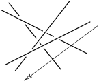
Figure 15. On the left, an amphicheiral interlacing of 4 lines. On the right, the same interlacing after sliding the uppermost two lines to the left and down. 8. Four Lines
9. Isotopic Lines of an Interlacing
Theorem 2.
By an isotopy one can make the lines of each equivalence class to belong to the same family of lines on a one-sheeted hyperboloid, and the hyperboloids containing the lines of the different equivalence classes to be disjoint. Theorem 3.
This invariant depends only on the class of lines isotopic to \(a\) and \(b\). Proof.
Lemma 1.
For any lines \(a,b,c,d\) one has Proof.
![]()
Lemma 2.
\(lk(a,b,x)\) does not depend on \(x\) when \(a\) and \(b\) are isotopic lines of the interlacing. Proof.
![]()
![]()
10. Five Lines
11. Six Lines
12. Seven Lines
13. Interlacings of Labeled Lines
14. Not Only Lines Can be Interlaced
Theorem 4.
A nonsingular set of \(q\) points in three-dimensional space is nonamphicheiral if \(q\equiv 6\mod 8\) or \(q\equiv 3\mod 4\) and \(q\ge 7\). Proof.
![]()
The following complete answer was found by Podkorytov [Podkorytov 1995] , after the previous version [Viro and Drobotukhina 1989] of this paper was written: Theorem 5 (Podkorytov Theorem) .
(See [Podkorytov 1995] .) An amphicheiral nonsingular set of \(q\) points and \(p\) lines in three-dimensional real projective space exists if and only if either 15. Plane Configurations of Lines
16. High-Dimensional Generalizations of Interlacings of Lines
17. Connection with Real Algebraic Surfaces of Degree \(4\)
References
9999999