Patchworking Algebraic Curves
Disproves the
Ragsdale Conjecture
Abstract
Real algebraic curves seem to be quite distant from combinatorial geometry. In this paper we intend to demonstrate how to build algebraic curves in a combinatorial fashion: to patchwork them from pieces which essentially are lines. One can trace related constructions back to Newton’s consideration of branches at a singular point of a curve. Nonetheless an explicit formulation does not look familiar for mathematicians outside of a narrow community of specialists in topology of real algebraic varieties.
This technique was developed by the second author in the beginning of eighties. Using it, the first author has recently found counter-examples to the oldest and most famous conjecture on the topology of real algebraic curves. The conjecture was formulated as early as 1906 by V. Ragsdale [14] on the basis of experimental material provided by A. Harnack’s and D. Hilbert’s constructions [5], [6].
1. Combinatorial Look on Patchworking
Initial Data. Let $m$ be a positive integer (it will be the degree of the curve under construction) and $T$ be the triangle in $\mathbb{R}^{2}$ with vertices $(0,0)$, $(m,0)$, $(0,m)$. Let $\tau$ be a triangulation of $T$ with vertices having integer coordinates and equipped with signs. The sign (plus or minus) at the vertex with coordinates $(i,j)$ is denoted by $\sigma_{i,j}$.
Construction of Piecewise Linear Curve. Take copies
| $T_{x}=s_{x}(T),\;\;T_{y}=s_{y}(T),\;\;T_{xy}=s(T)$ |
of $T$, where $s=s_{x}\circ s_{y}$ and $s_{x},\;s_{y}$ are reflections with respect to the coordinate axes. Denote by $T_{*}$ the square $T\cup T_{x}\cup T_{y}\cup T_{xy}$. Extend the triangulation $\tau$ to a symmetric triangulation of $T_{*}$, and the distribution of signs $\sigma_{i,j}$ to a distribution at the vertices of the extended triangulation by the following rule: $\sigma_{i,j}\sigma_{\varepsilon i,\delta j}\varepsilon^{i}\delta^{j}=1$, where $\varepsilon,\delta=\pm 1$. In other words, passing from a vertex to its mirror image with respect to an axis we preserve its sign if the distance from the vertex to the axis is even, and change the sign if the distance is odd.
If a triangle of the triangulation of $T_{*}$ has vertices of different signs, select a midline separating pluses from minuses. Denote by $L$ the union of the selected midlines. It is a collection of polygonal lines contained in $T_{*}$. The pair $(T_{*},L)$ is called the result of affine combinatorial patchworking. Glue by $s$ the sides of $T_{*}$. The resulting space $\mathcal{T}$ is homeomorphic to the real projective plane $\mathbb{R}P^{2}$. Denote by $\mathcal{L}$ the image of $L$ in $\mathcal{T}$ and call the pair $(\mathcal{T},\mathcal{L})$ the result of projective combinatorial patchworking.
Let us introduce an additional assumption: the triangulation $\tau$ of $T$ is convex. This means that there exists a convex piecewise-linear function $T\longrightarrow{\mathbb{R}}$ which is linear on each triangle of $\tau$ and not linear on the union of any two triangles of $\tau$.
1 Patchwork Theorem.
Under the assumptions above on the triangulation $\tau$ of $T$, there exist a nonsingular real algebraic plane affine curve of degree $m$ and a homeomorphism of the plane $\mathbb{R}^{2}$ onto the interior of the square $T_{*}$ mapping the set of real points of this curve onto $L$. Furthermore, there exists a homeomorphism $\mathbb{R}P^{2}\to\mathcal{T}$ mapping the set of real points of the corresponding projective curve onto $\mathcal{L}$.


2. Digression on Real Plane Algebraic Curves
The word curve is known to be one of the most ambiguous in mathematics. Thus it makes sense to specify the type of curve to be considered. The curves to be considered here are real algebraic plane curves, i. e. plane curves which are defined by equations $f=0$, where $f$ is a polynomial over the field $\mathbb{R}$ of real numbers. The constructions of curves, which we consider below, can be described as constructions of real polynomials $f(x,y)$ of a given degree such that the curves $f(x,y)=0$ are positioned in a complicated (for this degree) way in the plane $\mathbb{R}^{2}$.
However, for many reasons we prefer projective curves. To a reader who does not like (i. e. is not familiar with) the projective plane, we suggest the following motivations and definitions.
It was probably Isaac Newton [10] who first observed that a curve $f(x,y)=0$ in the plane $\mathbb{R}^{2}$ is a more complicated object (e. g., to classify) than the cone generated by it in $\mathbb{R}^{3}$. If $m$ is the degree of $f$, then the cone is defined by the equation $z^{m}f(x/z,y/z)=0$. Newton [10] found 99 classes of curves of degree 3 on $\mathbb{R}^{2}$, but at the end of his text noted that curves of all 99 classes can be obtained as plane sections of only 5 cubic cones.
In the nineteenth century this observation and similar ones led to the notion of the projective plane and the idea that it is simpler to study curves in the projective plane than in the affine plane.
The real projective plane $\mathbb{R}P^{2}$ can be defined as the set of lines in $\mathbb{R}^{3}$ passing through the origin $(0,0,0)$. The line passing through $(0,0,0)$ and $(x_{0},x_{1},x_{2})$ is denoted by $(x_{0}\colon x_{1}\colon x_{2})$; the numbers $x_{0}$, $x_{1}$, $x_{2}$ are called homogeneous coordinates of $(x_{0}:x_{1}:x_{2})$.
A cone in $\mathbb{R}^{3}$ with vertex $(0,0,0)$ can be viewed as a collection of lines lying on it. Since it is a one-parameter collection, it can be thought of as a curve in the projective plane. An equation $F(x,y,z)=0$, where $F$ is a homogeneous real polynomial, defines a cone in $\mathbb{R}^{3}$ with vertex $(0,0,0)$ and hence a curve in the projective plane $\mathbb{R}P^{2}$.
Take a curve on $\mathbb{R}^{2}$ defined by an equation $f(x,y)=0$ of degree $m$, shift it with its plane to the plane $z=1$ in $\mathbb{R}^{3}$ and consider lines passing through it and the origin $(0,0,0)$. These lines lie on the cone $z^{m}f(x/z,y/z)=0$ and fill it besides its intersection with the plane $x=0$. The corresponding curve on $\mathbb{R}P^{2}$ is called the projective completion of the affine curve $f(x,y)=0$. A study of real algebraic curves in the affine plane $\mathbb{R}^{2}$ is splits naturally into a study of their projective completions and an investigation of the position of the completions with respect to the line of infinity which is just the difference $\mathbb{R}P^{2}\smallsetminus\mathbb{R}^{2}$.
A curve (at least, an algebraic curve) is something more than just the set of points which belong to it. It is only slightly less than its equation: equations differing by a constant factor define the same curve. Modern algebraic geometry provides a lot of ways to define algebraic curve. Since we want to be as understandable as possible, we accept the following definition, which at first glance seems to be overly algebraic.
By a real projective algebraic plane curve of degree $m$ we mean a homogeneous real polynomial of degree $m$ in three variables, considered up to a constant factor. (Similarly, by a real affine algebraic plane curve of degree $m$ we mean a real polynomial of degree $m$ in two variables, considered up to a constant factor.) If $F$ is such a polynomial, then the equation $F(x_{0},x_{1},x_{2})=0$ defines the set of real points of the curve in the real projective plane $\mathbb{R}P^{2}$. Let $\mathbb{R}A$ denote the set of real points of the curve $A$. Following tradition, we also call this set a curve, avoiding this terminology only in cases where confusion could result.
A point $(x_{0}\colon x_{1}\colon x_{2})\in\mathbb{R}P^{2}$ is called a (real) singular point of the curve defined by a polynomial $F$ if the first partial derivatives of $F$ vanish in $(x_{0},x_{1},x_{2})$ (vanishing of the derivatives implies vanishing of the homogeneous polynomial: by the Euler formula $deg(F)\cdot F(x_{0},x_{1},x_{2})=\sum_{i}x_{i}\frac{\partial F}{\partial x_{i}% }(x_{0},x_{1},x_{2})$). A curve is said to be (real) nonsingular if it has no real singular points. The set $\mathbb{R}A$ of real points of a nonsingular real projective plane curve $A$ is a smooth closed one-dimensional submanifold of the projective plane. Then $\mathbb{R}A$ is a union of disjoint circles smoothly embedded in $\mathbb{R}P^{2}$. A circle can be positioned in $\mathbb{R}P^{2}$ either one-sidedly, like a projective line, or two-sidedly, like a conic. A two-sided circle is called an oval. An oval divides $\mathbb{R}P^{2}$ into two parts. The part homeomorphic to a disk is called the interior of the oval. Two ovals can be situated in two topologically distinct ways: each may lie outside the other one—i.e., each is in the outside component of the complement of the other—or else one of them is in the inside component of the complement of the other—in that case, we say that the first is the inner oval of the pair and the second is the outer oval. In the latter case we also say that the outer oval of the pair envelopes the inner oval. The topological type of the pair $(\mathbb{R}P^{2},\;\mathbb{R}A)$ is defined by the scheme of disposition of the ovals of $\mathbb{R}A$. This scheme is called the real scheme of curve $A$.
In 1900 D. Hilbert [7] included the following question in the 16-th problem of his famous list: what real schemes can be realized by curves of a given degree? The complete answer is known now only for curves of degree not greater than 7.
3. T-curves
Now let us come back to the Patchwork Theorem. It states that for any convex triangulation $\tau$ of $T$ with integer vertices and a distribution of signs at vertices of $\tau$ there exists a nonsingular real algebraic plane projective curve $A$ of degree $m$ such that the pair $(\mathbb{R}P^{2},\mathbb{R}A)$ is homeomorphic to the pair $(\mathcal{T},\mathcal{L})$ constructed as in Section 1, i. e. the result of projective combinatorial patchworking.
In fact, a polynomial defining the curve can be presented quite explicitly.
Construction of Polynomials. Given initial data $m$, $T$, $\tau$ and $\sigma_{i,j}$ as in Section 1 and a convex function $\nu$ certifying that the triangulation $\tau$ is convex. Consider a one-parameter family of polynomials
| $b_{t}(x,y)=\sum_{\begin{aligned}&{(i,j)\text{ runs over}}\\ &\text{ vertices of $\tau$}\end{aligned}}\sigma_{i,j}x^{i}y^{j}t^{\nu(i,j)}.$ |
Denote by $B_{t}$ the corresponding homogeneous polynomials:
| $B_{t}(x_{0},x_{1},x_{2})=x_{0}^{m}b_{t}(x_{1}/x_{0},x_{2}/x_{0}).$ |
Polynomials $b_{t}$ and $B_{t}$ are called the results of affine and projective polynomial patchworking.
2 Detailed Patchwork Theorem.
Let $m$, $T$, $\tau$, $\sigma_{i,j}$ and $\nu$ be initial data as above. Denote by $b_{t}$ and $B_{t}$ the non-homogeneous and homogeneous polynomials obtained by the polynomial patchworking of these initial data, and by $L$ and $\mathcal{L}$ the piecewise linear curves in the square $T_{*}$ and its quotient space $\mathcal{T}$ respectively obtained from the same initial data by the combinatorial patchworking.
Then there exists $t_{0}>0$ such that for any $t\in(0,t_{0}]$
-
(1)
$b_{t}$ defines an affine curve $a_{t}$ such that the pair $(\mathbb{R}^{2},\mathbb{R}a_{t})$ is homeomorphic to the pair $(T_{*},L)$ ;
-
(2)
$B_{t}$ defines a projective curve $A_{t}$ such that the pair $(\mathbb{R}P^{2},\mathbb{R}A_{t})$ is homeomorphic to the pair $(\mathcal{T},\mathcal{L})$ .
A curve obtained by this construction is called a T-curve.
All real schemes of curves of degree $\leq 6$ and almost all real schemes of curves of degree 7 have been realized by the patchwork construction described above. On the other hand, there exist real schemes realizable by algebraic curves of some (high) degree, but not realizable by T-curves of the same degree. Probably such a scheme can be found even for degree 7 or 8.
The construction of T-curves is a special case of more general patchwork construction, see [17] and [13]. In this generalization the patches are more complicated: they may be algebraic curves of any genus with arbitrary Newton polygon. Therefore the patches demand more care than above. This is why we restrict ourselves here to T-curves. However, even constructing T-curves it is useful to think in terms of blocks more complicated than a single triangle (made of several triangles).
The rest of the paper is devoted to applications of the patchwork construction.
4. Ragsdale Conjecture
As far as we know, until 1876 no specific result was obtained concerning the topology of nonsingular real plane curves of an arbitrary degree. The year 1876 is often considered as the beginning of the topological study of real algebraic curves. Prior to that topological properties were not separated from other geometric properties, which are more subtle and could keep geometers busy with curves of a few lower degrees.
In 1876 A. Harnack published a paper [5] where he found an exact upper bound for the number of components for a curve of a given degree. Harnack proved that the number of components of a real plane projective curve of degree $m$ is at most $\frac{(m-1)(m-2)}{2}+1$. On the other hand, for any natural number $m$ he constructed a nonsingular real projective curve of degree $m$ with $\frac{(m-1)(m-2)}{2}+1$ components, which shows that his estimate cannot be improved without introducing new ingredients.
It was D. Hilbert who made the first attempt to study systematically topology of nonsingular real plane algebraic curves. The first difficult special problems he met were related to curves of degree 6.
Hilbert suggested that from a topological viewpoint the most interesting are the curves having the maximal number $\frac{(m-1)(m-2)}{2}+1$ of components among curves of a given degree $m$. Hilbert’s guess was strongly confirmed by the whole subsequent development of the field. Now, following I. Petrovsky, these curves are called M-curves.
Hilbert succeeded in constructing M-curves of degree $\geq 6$ with mutual position of components different from the ones realized by Harnack. However he realized only one new real scheme of degree 6. See Figure [4] where the real schemes of Harnack’s and Hilbert’s curves of degree 6 are shown. Hilbert conjectured that these are the only real schemes realizable by M-curves of degree 6 and for a long time claimed that he had a (long) proof of this conjecture. Even being false (it was disproved by D. A. Gudkov in 1969, who constructed a curve with the real scheme shown in Figure 5) this conjecture captured the essence of what in the 30-th and 70-th became the core of the theory.


In fact, Hilbert invented a method which allows one to answer all questions on the topology of curves of degree 6. It involves a detailed analysis of singular curves which could be obtained from a given nonsingular one. The method required complicated fragments of singularity theory, which had not been elaborated at the time of Hilbert. It was only in the sixties that this project was completely realized. A complete table of real schemes of curves of degree 6 was obtained by Gudkov.
Coming back to Hilbert, we should mention his famous list of problems [7]. He included in the list, as a part of the sixteenth problem, a general question on topology of real algebraic varieties and more special questions like the problem on the mutual position of components of a plane curve of degree 6.
One curious aspect of this problem seems to be its number in the list. The number sixteen plays a very special role in the topology of real algebraic varieties. It is difficult to believe that Hilbert was aware of that. It became clear only in the beginning of seventies (see Rokhlin’s paper “Congruences modulo 16 in Hilbert’s sixteenth problem” [15]). Nonetheless, sixteen was the number assigned by Hilbert to the problem.
In 1906 V. Ragsdale [14] made a remarkable attempt to analyze Harnack’s and Hilbert’s constructions to guess new restrictions on topology of curves. To a great extent the success of her analysis was due to the right choice of parameters of a real scheme.
Ragsdale suggested considering separately the case of curves of even degree $m=2k$. Each connected component of the set of real points of a curve of even degree is an oval (i. e., positioned in $\mathbb{R}P^{2}$ two-sidedly and divides $\mathbb{R}P^{2}$ into two parts). An oval of a curve is called even (resp. odd) if it lies inside of an even (resp. odd) number of other ovals of this curve. The number of even ovals of a curve is denoted by $p$, the number of odd ovals by $n$.
It was Ragsdale who suggested distinguishing even and odd ovals. Ragsdale provided good reasons why one should pay special attention to $p$ and $n$. A curve of an even degree divides the plane $\mathbb{R}P^{2}$ into two pieces with a common boundary $\mathbb{R}A$ (these pieces are the subsets of $\mathbb{R}P^{2}$ where a polynomial defining the curve takes positive and negative values, respectively). One of these pieces is nonorientable, it is denoted by $\mathbb{R}P^{2}_{-}$. The other one is denoted by $\mathbb{R}P^{2}_{+}$. The numbers $p$ and $n$ are the fundamental topological characteristics of $\mathbb{R}P^{2}_{+}$ and $\mathbb{R}P^{2}_{-}$. Namely, $p$ is the number of connected components of $\mathbb{R}P^{2}_{+}$, and $n+1$ is the number of connected components of $\mathbb{R}P^{2}_{-}$ (exactly one component of $\mathbb{R}P^{2}_{-}$ is nonorientable, so $n$ is the number of orientable components of $\mathbb{R}P^{2}_{-}$). Ragsdale singled out also the difference $p-n$ motivating this by the fact that it is the Euler characteristic of $\mathbb{R}P^{2}_{+}$. It is amazing that essentially these considerations were stated in a paper in 1906!
3 Ragsdale Observation.
For any of Harnack’s $M$-curves of even degree $m=2k$,
| $p=\frac{3k(k-1)}{2}+1,\qquad n=\frac{(k-1)(k-2)}{2}.$ |
For any of Hilbert’s $M$-curves of even degree $m=2k$,
| $\displaystyle\frac{(k-1)(k-2)}{2}+1\leq p\leq\frac{3k(k-1)}{2}+1,$ | ||
| $\displaystyle\frac{(k-1)(k-2)}{2}\leq n\leq\frac{3k(k-1)}{2}.$ |
This motivated the following conjecture.
4 Ragsdale Conjecture.
For any curve of even degree $m=2k$,
| $p\leq\frac{3k(k-1)}{2}+1,\qquad n\leq\frac{3k(k-1)}{2}.$ |
Writing cautiously, Ragsdale formulated also weaker conjectures. About thirty years later I. G. Petrovsky [11], [12] proved one of these weaker conjectures.
5 Petrovsky Inequalities.
For any curve of even degree $m=2k$,
| $p-n\leq\frac{3k(k-1)}{2}+1,\qquad n-p\leq\frac{3k(k-1)}{2}.$ |
It is clear from [11] and [12], that Petrovsky was not familiar with Ragsdale’s paper. But his proof runs along the lines indicated by Ragsdale. He also reduced the problem to estimates of the Euler characteristic of the pencil curves, but he went further: he proved these estimates using the Euler-Jacobi formula.
Petrovsky also formulated conjectures about the upper bounds for $p$ and $n$. His conjecture about $n$ was more cautious (by 1).
Both the Ragsdale Conjecture formulated above and its version stated by Petrovsky [12] are wrong. However they stood for a rather long time: the Ragsdale Conjecture for $n$ was disproved by O. Y. Viro [16] in 1979. Viro’s disproof looked rather like an improvement of the conjecture, since in the counter-examples $n=\frac{3k(k-1)}{2}+1$. In 1993 Ragsdale-Petrovsky bounds were disproven by a considerable margin in I. V. Itenberg [8]: in Itenberg’s counter-examples the difference between $p$ (or $n$) and $\frac{3k(k-1)}{2}+1$ is a quadratic function of $k$ (see below).
The numbers $p$ and $n$ introduced by Ragsdale occur in many of the prohibitions that were subsequently discovered. While giving full credit to Ragsdale for her insight, we must also say that, if she had looked more carefully at the experimental data available to her, she should have been able to find some of these prohibitions. For example, it is not clear what stopped her from making the conjectures which were made by Gudkov [2] in the late 1960’s. In particular, the experimental data could suggest the formulation of the Gudkov-Rokhlin congruence [15]: for any M-curve of even degree $m=2k$
| $p-n\equiv k^{2}\mod 8$ |
Maybe mathematicians trying to conjecture restrictions on some integer should keep this case in mind as evidence that restrictions can have not only the shape of an inequality, but a congruence. Proof of these Gudkov’s conjectures initiated by Arnold [1] and completed by Rokhlin [15], Kharlamov [9], Gudkov and Krakhnov [3] marked the beginning of the most recent stage in the development of the topology of real algebraic curves.
Which of Ragsdale’s questions are still open now? The inequalities
| $p\leq\frac{3k(k-1)}{2}+1,\qquad n\leq\frac{3k(k-1)}{2}+1$ |
have been neither proved nor disproved for $M$-curves. Ragsdale gave interesting reformulations of the first of these inequalities for $M$-curves. Below we present her reformulations together with the corresponding reformulations of the inequality $n\leq\frac{3k(k-1)}{2}+1$.
6 Ragsdale Conjecture on M-curves.
For any $M$-curve of degree $2k$
| $|p-n|\leq k^{2},$ |
or, equivalently,
| $p\geq\frac{(k-1)(k-2)}{2}\quad\text{ and }\quad n\geq\frac{(k-1)(k-2)}{2}\quad.$ |
5. Patchworking Harnack Curves
In each area of mathematics there are objects which appear much more frequently than other ones. Some of them (like Dynkin diagrams) appear in several domains quite distant from each other. In topology of real plane algebraic curves Harnack curves play this role. It was not an accident that they were constructed in the first paper devoted to this subject. Whenever one tries to construct an M-curve, the first success provides a Harnack curve. Patchwork construction is no exception to the rule.
In this section we describe, using the Patchwork Theorem, the construction of some Harnack curves of an even degree $m=2k$.
In what follows all the triangulations satisfy an additional assumption: they are primitive which means that all triangles are of area 1/2 (or, equivalently, that all integer points of the triangulated area are vertices of the triangulation). A polynomial defining a T-curve contains the maximal collection of nonzero monomials if and only if the triangulation used in the construction of the T-curve is primitive.
A primitive convex triangulation of $T$ is said to be equipped with a Harnack distribution of signs if:
vertex $(i,j)$ has the sign ”-”, if $i,j$ are both even, and has the sign ”+” in the opposite case.
A vertex $(i,j)$ of a triangulation of $T$ is called even if $i,j$ are both even, and odd if not.

Proposition 7.
Patchworking applied to an arbitrary primitive convex triangulation of $T$ with the Harnack distribution of signs produces an M-curve with the real scheme shown in Figure 6.
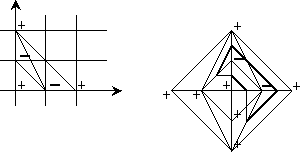
An example of the construction under consideration is shown in Figure 7.

Proof of Proposition. First, remark that the number of interior (i. e., lying in the interior of the triangle $T$) integer points is equal to $\frac{(m-1)(m-2)}{2}$, the number of even interior points is equal to $\frac{(k-1)(k-2)}{2}$, and the number of odd interior points is equal to $\frac{3k(k-1)}{2}$.
Take an arbitrary even interior vertex of a triangulation of the triangle $T$. This vertex has the sign ”-”. All adjacent vertices (i.e. the vertices connected with the vertex by edges of the triangulation) are odd, and thus they all have the sign ”+”. This means that the star of an even interior vertex contains an oval of the curve $L$. The number of such ovals is equal to $\frac{(k-1)(k-2)}{2}$.
Take now an odd interior vertex of the triangulation. It has the sign ”+”. There are two vertices with ”-” and one vertex with ”+” among the images of the vertex under $s=s_{x}\circ s_{y}$ and $s_{x},\;s_{y}$ (recall that $s_{x},\;s_{y}$ are reflections with respect to the coordinate axes). Consider the image with the sign ”+”. It is easy to verify, that all its adjacent vertices have the sign ”-”. Again this means that the star of this vertex contains an oval of the curve $L$. The number of such ovals is equal to $\frac{3k(k-1)}{2}$.
Thus
| $\frac{(k-1)(k-2)}{2}\;+\;\frac{3k(k-1)}{2}\;=\;\frac{(m-1)(m-2)}{2}$ |
so the curve can only have one more oval. This oval exists, because, for example, the curve $L$ intersects the coordinate axes.
To finish the proof, we need only note that the union of the segments
| $\{x-y=-m,\;-m\leq x,y\leq m\}\;\;\cup$ |
| $\{x\leq 0,\;y=0,\;-m\leq x,y\leq m\}\;\;\cup\;\;\{x=0,\;y\leq 0,\;-m\leq x,y% \leq m\}$ |
is not contractible in $\mathcal{T}$ and contains only minuses. This means that $\frac{3k(k-1)}{2}$ ovals corresponding to odd interior points and encircling pluses are situated outside of the nonempty oval. ∎
6. Counter-Examples to Ragsdale Conjecture
The following theorem gives counter-examples to the Ragsdale Conjecture (or the conjecture of Petrovsky) (cf. [8]).
Theorem 8.
For each integer $k\geq 1$
a) there exists a nonsingular real algebraic plane projective curve of degree $2k$ with
| $p=\frac{3k(k-1)}{2}+1+\left[\frac{(k-3)^{2}+4}{8}\right]$ |
b) there exists a nonsingular real algebraic plane projective curve of degree $2k$ with
| $n=\frac{3k(k-1)}{2}+\left[\frac{(k-3)^{2}+4}{8}\right]$ |
Remarks
The term $\left[\frac{(k-3)^{2}+4}{8}\right]$ is positive when $k\geq 5$ (i. e., the first counter-examples to the Ragsdale Conjecture appear in degree 10; the patchwork of them is shown in Figures 2 and 3). On the other hand, it is known that there is no counter-example to the Ragsdale Conjecture among curves of lower degree. These counter-examples of degree 10 have the real schemes shown in Figure 8. One of these counter-examples can be improved in order to obtain a curve of degree 10 with $n=32$. The corresponding patchworks (for $p=32$ and $n=32$) are shown in Figures [2] and [3].

Recently B. Haas [4] improved the construction presented below and obtained T-curves of degree $2k$ with
| $p=\frac{3k(k-1)}{2}+1+\left[\frac{k^{2}-7k+16}{6}\right].$ |
Neither the counter-examples provided by the above theorem, nor curves constructed by Haas are M-curves. Moreover, as we mentioned above, it is not known if the conjecture of Petrovsky holds for M-curves. The only known counter-examples to the Ragsdale Conjecture among M-curves are the curves constructed by Viro [16] (see also [18]). It is curious that we did not succeed in presenting those M-counter-examples as T-curves.
Proof.
Proof of Theorem Let us show, first, how to construct a curve of degree $m=2k$ with $p=\frac{3k(k-1)}{2}+2$.
Suppose that the hexagon $S$ shown in Figure 9 is placed inside of the triangle $T$ in such a way that the center of $S$ has both coordinates odd. Any convex primitive triangulation of a convex part of a convex polygon is extendable to a convex primitive triangulation of the polygon. Inside of the hexagon $S$, let us take the convex primitive triangulation shown in Figure 9 and extend it to $T$.

To apply the Patchwork Theorem we need to choose signs at the vertices. Inside of $S$ put signs according to Figure 9; outside use the Harnack rule of distribution of signs.
It is easy to calculate that the corresponding piecewise-linear curve $\mathcal{L}$ has exactly one even oval more than the Harnack curve constructed above (i. e. now $p=\frac{3k(k-1)}{2}+2$). One can verify that the curve obtained has the real scheme shown in Figure 10.

Consider the partition of the triangle $T$ shown in Figure 11. Let us take in each shadowed hexagon the triangulation and the signs of the hexagon $S$. The triangulation of the union of the shadowed hexagons can be extended to the primitive convex triangulation of $T$. Let us fix such an extension. Outside of the union of the shadowed hexagons choose the signs at the vertices of the triangulation using the Harnack rule.

Calculation shows that for the corresponding piecewise-linear curve $\mathcal{L}$
| $p=\frac{3k(k-1)}{2}+1+a$ |
where $a$ is the number of shadowed hexagons, and
| $a=\left[\frac{(k-3)^{2}+4}{8}\right]$ |
This curve has the real scheme shown in Figure 12.

To prove part b) of the theorem, let us take again the partition of the triangle $T$ shown in Figure [11] with the triangulation and the signs of each shadowed hexagon coinciding with the triangulation and the signs of $S$. Fix, in addition, a triangulation of a neighborhood of the axis $OY$ and the signs at the vertices of the triangulation as shown in Figure 13 (the case $k\equiv 1(\mod 4)$). The chosen triangulation of the union of the shadowed hexagons and the neighborhood of the $y$-axis can be extended to a primitive convex triangulation of $T$. Outside of the union of the shadowed hexagons and the neighborhood of the $y$-axis let us again choose the signs at the vertices of the triangulation using the Harnack rule.

The corresponding piecewise-linear curve $\mathcal{L}$ has the real scheme shown in Figure 14. In this case $n=\frac{3k(k-1)}{2}+a$. ∎

References
- 1 V. I. Arnold, On the location of ovals of real algebraic plane curves, involutions on four-dimensional smooth manifolds, and the arithmetic of integral quadratic forms, Funktsional. Anal. i Prilozhen 5 (1971), 1–9 (Russian), English translation in Functional Anal. Appl. 5 (1971), 169–176.
- 2 D. A. Gudkov and G. A. Utkin, The topology of curves of degree 6 and surfaces of degree 4, Uchen. Zap. Gorkov. Univ., vol. 87, 1969 (Russian), English transl., Transl. AMS 112.
- 3 D. A. Gudkov and A. D. Krakhnov, On the periodicity of the Euler characteristic of real algebraic $(M-1)$-manifolds, Funktsional. Anal. i Prilozhen. 7 (1973), 15–19 (Russian), English translation in Functional Anal. Appl. 7 (1971).
- 4 B. Haas, Les multilucarnes: Nouveaux countre-exemples à la conjecture de Ragsdale, (to appear in C. R. Acad. Sci. Paris).
- 5 A. Harnack, Über Vieltheiligkeit der ebenen algebraischen Curven, Math. Ann. 10 (1876), 189–199.
- 6 D. Hilbert, Über die reellen Züge algebraischen Curven, Math. Ann. 38 (1891), 115–138.
- 7 D. Hilbert, Mathematische Probleme, Arch. Math. Phys. 3 (1901), 213–237 (German).
- 8 I. Itenberg, Countre-ememples à la conjecture de Ragsdale, C. R. Acad. Sci. Paris 317, Serie I (1993), 277–282.
- 9 V. M. Kharlamov, New congruences for the Euler characteristic of real algebraic varieties, Funktsional. Anal. i Prilozhen. 7 (1973), 74–78 (Russian), English translation in Functional Anal. Appl. 7 (1973).
- 10 I. Newton, Enumeratio linearum tertii ordinis, London (1704).
- 11 I. Petrovsky, Sur le topologie des courbes réelles et algèbriques, C. R. Acad. Sci. Paris (1933), 1270–1272.
- 12 I. Petrovsky, On the topology of real plane algebraic curves, Ann. of Math. 39 (1938), 187–209.
- 13 J.-J. Risler, Construction d’hypersurfaces réelles (d’après Viro), Séminaire N. Bourbaki (1992), no. 763.
- 14 V. Ragsdale, On the arrangement of the real branches of plane algebraic curves, Amer. J. Math. 28 (1906), 377–404.
- 15 V. A. Rokhlin, Congruences modulo 16 in Hilbert’s sixteenth problem, Funktsional. Anal. i Prilozhen. 6 (1972), 58–64 (Russian), English translation in Functional Anal. Appl. 6 (1972), 301–306.
- 16 O. Ya. Viro, Curves of degree 7, curves of degree 8 and the Ragsdale conjecture, Dokl. Akad. Nauk SSSR 254 (1980), 1305–1310 (Russian), English translation in Soviet Math. Dokl. 22 (1980), 566–570.
- 17 O. Viro, Gluing of plane real algebraic curves and constructions of curves of degrees 6 and 7 Lecture Notes in Math. 1060 (1984), Springer-Verlag, 187–200.
- 18 O. Ya. Viro, Plane real algebraic curves: constructions with controlled topology, Algebra i analiz 1 (1989), 1–73 (Russian), English translation in Leningrad Math. J. 1:5, 1990, 1059–1134.
